About Skew-T Log-P Charts

A skew-t log-p chart plots the temperature, dew point and winds above a specific point on the ground. For example, the following skew-t log-p chart illustrates the atmosphere above Oshkosh from ground level up to 45,000 feet on the y-axis.  The x-axis includes the temperature which is skewed to the right at a 45-degree angle. The thin red line that travels upward to the right from the 0 degree tick up to a pressure altitude of about 27,000 feet is called an isotherm. The thick red line plots the temperature at various altitudes. The thick blue line plots the dew point at various altitudes. In this example, the dew point and temperature are converging between 4,000 and 5,000 feet which indicates saturation of the air and thus, clouds. Since these clouds are to the right of the 0-degree isotherm they are below freezing which means icing is a possibility. This particular chart would tell the non-FIKI pilot to stay below 5,000 feet in this area.

Winds aloft are depicted on the right side of the chart. The red barbs indicate the direction and velocity of the wind at a specific pressure altitude. In this example, the winds begin shifting from the west to the southeast at around 15,000 feet and back to the west at around 25,000 feet. To the right of the barbs is a thin blue line depicting the wind velocity in knots.

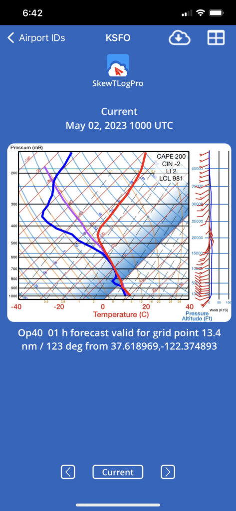
Here is the METAR for KSFO available at the time of this chart indicating a broken layer at 4,100 feet:

KSFO 020956Z 23007KT 10SM FEW028 BKN041 11/07 A2976 RMK AO2 SLP076 T01110072

The thick purple line is the lifted parcel line, also known as the LPL or simply the parcel line, which represents the temperature profile of an air parcel as it rises adiabatically through the atmosphere. It is an important concept in meteorology, as it helps determine atmospheric stability and the potential for convective development, such as thunderstorms or other severe weather events.

To construct the lifted parcel line, meteorologists usually start by identifying the temperature and dew point temperature of a surface air parcel (often taken from surface observations). Then, they assume the parcel is lifted vertically from the ground, rising adiabatically, without any heat exchange with its surroundings. As the air parcel rises, it cools at the dry adiabatic lapse rate until it reaches its lifting condensation level (LCL), where the dew point temperature equals the air temperature and condensation begins. Above the LCL, the parcel continues to rise, but now it cools at the moist adiabatic lapse rate due to the release of latent heat during condensation.

On a Skew-T Log-P chart, the lifted parcel line is drawn by connecting the temperature points for the rising air parcel at different pressure levels (or altitudes). The LPL is then compared to the environmental temperature profile (usually plotted in red) to assess atmospheric stability. If the LPL is warmer than the environmental temperature at a certain altitude, it indicates the parcel is buoyant and will continue to rise, suggesting an unstable atmosphere. Conversely, if the LPL is cooler than the environmental temperature, the parcel will sink, indicating a stable atmosphere.

The skew-t log-p chart was invented in 1947 as a tool for the United States Air Force to evaluate the atmosphere. According to Wikipedia:

“In 1947, N. Herlofson proposed a modification to the emagram which allows straight, horizontal isobars, and provides for a large angle between isotherms and dry adiabats, similar to that in the tephigram. It was thus more suitable for some of the newer analysis techniques being invented by the United States Air Force.”

Here are some recommended resources for learning more about skew-t log-p charts:

• IFR Magazine: Reading a Skew-T Log(P) Part I by Scott Dennstaedt
• IFR Magazine: Reading a Skew-T Log(P) Part II by Scott Dennstaedt
• IFR Magazine: Reading a Skew-T Log(P) Part III by Scott Dennstaedt

SkewTLogPro costs $17.99 in the Apple app store.

SkewTLogPro will run on all iPhone and iPad devices. An Android version is not currently available.

Yes, you can run SkewTLogPro on all of your devices using a single Apple ID.

The continental US and Canada are supported with data from the Op40 model. The rest of the world is supported with data from the GFS model.

SkewTLogPro uses data from NOAA at http://rucsoundings.noaa.gov/